

Accurately measuring price elasticity in retail is key to any pricing optimization effort. Managers and online retailers need to understand the microeconomics of how customers respond to a price change in order to realize the full potential of pricing and price elasticity.

Using price elasticity, businesses can:

  • Identify products that are important to your customers and therefore critical to building your price image
  • Identify products for which your customers regularly compare prices
  • Calculate profit and revenue scenarios for different price points of a single item or for a quantity of items, or your entire assortment
  • Create a demand function and chart a demand curve
  • Design an automated, optimized, and demand-driven pricing strategy

So what is price elasticity? How is it measured, and how is it used for price optimization?

In this webinar, 7Learnings Co-Founder Eiko van Hettinga breaks down the core microeconomic principles behind price elasticity and explains how retailers can quantify how customers truly react to price changes.

What is price elasticity?

Price elasticity measures how demand for a product changes after a price adjustment. It can be calculated with a mathematical formula to produce a demand function, represented as a demand curve, which shows how often a product is sold at what price. 

At the same time, the demand function can be used to determine how the demand for an item changes when the price is adjusted. Accordingly, it is a matter of the price elasticity of demand.

Most customers and most markets are sensitive to price changes. A price increase usually leads to a decrease in demand because customers do not want to spend more money on a product or service. A price decrease, on the other hand, usually leads to an increase in demand. This is called price elasticity because it can fluctuate depending on the price.

Demand curve graph with price elasticity of demand formula.
Demand curve & formula to calculate price elasticity of demand

Why price elasticity is hard to measure — and how ML solves it

Measuring price elasticity is difficult because companies do not generally operate under ideal test conditions. Often, not only are prices adjusted, but other internal and external factors that influence price elasticity, such as competitor prices or the weather (and thus demand), are changing at the same time. 

Price elasticities are not constant along the entire price-demand curve. Good elasticities in particular tend to vary along the demand curve, and will typically tend to be higher (in absolute terms) near the prices of major competitors.

As it is not easy to measure price elasticity, many retailers resort to simpler methods of pricing. Often, they work with simple rule-based methods built from “if then” conditions. However, leading retailers are not satisfied with this and use price elasticities as a basis for pricing. 

To calculate these, machine learning-based algorithms are used, which, in a first step, measure the effect of price changes on sales. These algorithms also take into account a much higher number of other factors that affect customers’ willingness to pay. 

More accurate price optimization based on the calculation of price elasticities leads to a significant increase in profit. In online retailing, companies such as 7Learnings have been able to prove this increase in profit using A/B tests.

The harder problem is scale. To learn elasticity reliably at the individual product level, a retailer needs enough sales at enough different price points — data that best-sellers generate but most of the assortment does not. Low-selling products simply never sell at enough distinct prices for a manual analysis to reach a dependable figure on their own. 

This is the structural reason rule-based methods persist: they are manageable by hand, but they cap how precise pricing can become, because a rule cannot reason about demand. Machine learning changes what is measurable. 

By learning elasticity across clusters of similar products, an item with little price history inherits signals from comparable products that have more, drawing on the same demand forecasting methods now common in retail. 

The model can also weigh the full range of signals that move willingness to pay, including competitor prices, weather, seasonality, product life cycle stage, and a shopper’s position in the cart among them.

Calculating the price elasticity of demand

When it comes to most products, consumers are sensitive to price changes and would buy less when the price increases. The price elasticity is then negative. Positive price elasticity occurs when a higher price leads to higher demand, which is rather rare and more likely the case in the luxury segment. 

To compare different goods and services, the price elasticity of demand is calculated by dividing the percentage change in demand by the percentage change in price:

Price elasticity of demand formula: dQ/Q divided by dP/P.

PED (price elasticity of demand) = (change in demand/change in price)

When price elasticity is high, demand is strongly related to price, as in the case of consumer goods of certain brands (e.g., a certain yogurt or a branded sneaker). When price elasticity is low, demand and price are hardly related, as in the case of essential goods. For example, basic groceries, gasoline, or housing. Low price elasticity is also the case when there are no substitute products. 

Even with price increases, demand then remains relatively stable, which is referred to as price inelasticity. Thus, it is also important for price elasticity whether equivalent substitute products or substitute goods are available.

For the demand function formula, this means that price elasticities in the retail sector are almost always negative: Demand is said to be elastic if the value of elasticity is above 1, and inelastic if it is below 1.

Price elasticity in trade: an example

We’ll apply the price elasticity formula to an online retailer of TV sets. The retailer decides to lower the price of Brand X TV sets from 1,000 euros to 750 euros and assumes that this will increase the quantity of sales from 10,000 brand X TV sets to 20,000 sets per month.
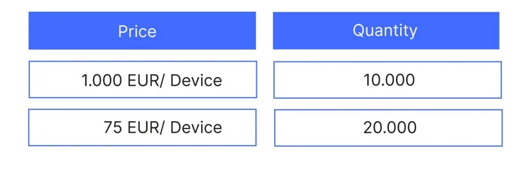
Table showing device prices and quantities in Euros.
Calculating the price elasticity

To calculate price elasticity, we look at the percentage change in quantity demanded and the percentage change in price:

% change in price = (750 euros – 1,000 euros) / (1,000 euros) = -25%

% change in demand = (20,000 – 10,000) / (10,000) = +100%

From this follows: the price elasticity = 100% / -25% = -4

This means that demand is relatively elastic: sales of the TV will change greatly if the retailer changes the price, whether up or down. The product is thus highly competitive for the retailer. If demand were not very elastic, a price change would have little effect on sales figures, and the product would have little competitive relevance. 

The formula works the same way regardless of currency or retail category: the same calculation applies whether prices are in dollars or euros, and whether the product is a TV set or a jacket.

Different types of price elasticity of demand

TypesWhat is it?Effect on Revenue

Perfectly Inelastic Demand,

(PED = 0)

  • No change in demand for a change in price.
  • Demand remains constant for any value of price.
  • The demand curve is shown as a straight vertical line.
  • There is no product that has perfectly inelastic demand – most likely essential goods such as water, housing, or basic food items.
Price ↑     Revenue ↑
Price ↓      Revenue ↓

Relatively Inelastic Demand,

(PED = 0 <x <1)

  • The percentage change in demand is less than the percentage change in price.
  • The demand curve is rapidly increasing.
  • A typical example is gasoline.
Price ↑    Revenue ↑
Price ↓    Revenue ↓

Unit Elastic Demand,

(PED = 1)

  • The proportional change in demand causes the same change in price.
  • The quantity demanded changes by the same percentage as the price change.
  • This can affect different products and services depending on the market situation, e.g. electricity (suppliers).

Price ↑ then

No Change in Total Revenue

Price ↓ then

No Change in Total Revenue

Relatively Elastic Demand,

(PED = 1< x<∞)

  •  The generated proportional change in demand is greater than the proportional change in price.
  • The quantity demanded changes by a greater percentage than the change in price.
  • The demand curve is shown to rise gradually. It is less steep than relatively inelastic demand.
  • Many consumer goods fall into this range.

Price ↑    Revenue ↓

Price ↓    Revenue ↑

 Perfectly Elastic Demand,

(PED = ∞)

  • A small increase in price causes demand to fall to zero, while a small decrease in price causes demand to become infinite.
  • Consumers buy everything available at a given price, but nothing at any other price.
  • This is a theoretical concept because it assumes perfect competition, where the smallest price increase leads to zero demand.

Price ↑ then 0 total Revenue 

Preis ↓ then 0 total Revenue

Cross-price elasticity and cannibalization in retail

Price elasticity measures the effect of price changes of one product on its own sales. But this is not the only relevant elasticity, as there are also interdependencies between products. These interdependencies are measured by cross-price elasticity. 

Cross-price elasticity of demand measures the percentage sales modification of a particular product that is demanded, relative to the change in the price of another product. In real-world scenarios, this can be seen in how the price changes of certain products impact the demand for others. It can also measure either complementary products or substitute products. Being able to measure this can help retailers make informed decisions about their product assortments and the prices they set against their range. 

A negative cross price elasticity means that the two products are substitutes for one another, and the increase in price for one would lead to higher consumer demand for the other. Conversely, a product complement exists when the increase in the price of product #1 leads to a decrease in the demand for product #2, as the two products are used in conjunction with one another.

A practical example of cross price elasticity for complementary products would be a decrease in the price of hot dogs, which would lead to an increase in the demand for hot dog buns. This would be considered a positive cross price elasticity of demand. This method is often used strategically by retailers in this scenario to encourage sales of complementary products.

A common example of substitute products in cross price elasticity would be toothpaste. If the price of one brand of toothpaste increases, the demand for other brands of competing toothpaste would increase.

In fashion and apparel, this shows up most sharply as cannibalization. When a retailer marks down one colorway of a style, the discounted variant often pulls demand away from its full-price sibling SKUs rather than only bringing in new buyers. 

Understanding that relationship is what separates a markdown that clears slow stock from one that quietly erodes full-price sales across the style. The same logic can work in the retailer’s favor: products that are very cross-elastic (e.g., different pack sizes of the same product) can be priced together as a coherent set rather than in isolation.

What affects price elasticity in fashion and apparel retail

The price elasticity of a product is influenced by many factors. It is often not easy to identify them and measure their effect on price elasticity. In addition, factors change and therefore price elasticity does not have a constant value over time. The following items often have a direct impact on the price elasticity of an item or service:

Type of product:

The price elasticity of a product is influenced by many factors that are hard to identify and measure. And since those factors change, elasticity itself changes over time. Here’s what typically affects it:

Type of product — necessary goods vs. luxury goods

  • Goods that are essential to life are usually inelastic, meaning that a price change has little effect on demand. For example, if the price of gasoline goes up, demand doesn’t change much because people still need to use their cars to get to work.
  • Textbooks or prescription drugs.
  • Products that show more price elasticity make life more enjoyable, such as a television or a gym membership.
  • In the case of pleasure and luxury goods such as a sports car or a diamond ring, taste also plays a role. These products are basically not essential to life.

Income and economy

  • The average income of a consumer group or an economy also influences the price elasticity of demand for goods and services.
  • If the economy is in a downturn, the decline in annual income for the majority of the population may cause luxury items to have more price elasticity.
  • A recession causes consumers to save rather than spend money on luxury items.

Competition and substitutes

  • The more competition or the higher the quantity of substitute products, the more elastic demand is because consumers can easily switch.
  • For example, if the price of Bavarian asparagus has increased due to bad weather and poor harvest, but asparagus from Spain is an equivalent competing product in taste, quality, and price, then consumer demand for it will increase.

Product life cycle and seasonal assortment

  • For new products, the price elasticity of demand is low because there is little or no competition in the market.
  • In contrast, the long-tail SKUs or items with price discounts have more price elasticity.
  • In fashion, this is amplified by the seasonal calendar: the same garment can behave very differently at the start of a season, mid-season, and during end-of-season clearance, which is part of what makes seasonal assortments so demanding to price.

Level of price

  • For most products, price elasticity is not the same for all prices.
  • Often, high-priced products have more price elasticity because customers put more thought into the purchase and investment. They are also more likely to compare prices with competing products.

Retailer brand and service

  • The price elasticity of a product interacts with the rest of a retailer’s offering.
  • If, for example, a retailer offers a bonus program or particularly good delivery conditions, customers are less likely to switch and will buy even if prices are higher, thus reducing price elasticity.
  • A retailer’s brand can also have a positive or negative impact on price elasticity.

Channel — marketplace vs. own website

  • The same product often carries different elasticity depending on where it sells. On a marketplace, shoppers can compare competing offers side by side within seconds, so demand tends to be more price-sensitive and more elastic.
  • On a retailer’s own website, where the comparison set is narrower and the brand relationship stronger, the same item can be noticeably less elastic. Pricing both channels with a single rule ignores that difference.

Promotional vs. clearance elasticity

  • A single item does not have one elasticity; it has several, depending on the pricing context. The elasticity of a garment at full price, on promotion, and in clearance are different coefficients for the same SKU.
  • A shopper who ignores a small in-season markdown may respond strongly to a clearance discount on the identical product weeks later. Treating these as one number is a common source of margin leakage, and the distinction is directly relevant to the markdown and sell-through decisions at the core of fashion pricing.

This list of factors is not exhaustive. Many other points, such as the position in the shopping cart, can influence price elasticity.

Tariffs and cost pass-through

Tariffs have become a live pricing question for US apparel retailers. The average tariff rate on US apparel imports (HS chapters 61 and 62) rose from 14.7% in December 2024 to 35.1% in December 2025. 

When input costs jump like this, a blanket price increase ignores which SKUs have pricing power and which don’t: inelastic products can absorb an increase with little volume loss, while elastic ones cannot, and an across-the-board move risks crossing price thresholds that trigger customer backlash.

An elasticity-driven approach handles this differently. In a documented example, Oliver Wyman worked with a specialty retailer that had reacted to earlier tariffs with broad, sub-5% increases across tens of thousands of SKUs, crossed price thresholds, and lost sales it never recovered. 

Using elasticity to target its moves (larger increases on a focused set of 4,000 SKUs with pricing power, plus price investment on around 200 where it was needed), the retailer achieved a 9% margin increase while growing sales 5%. For apparel retailers facing cost pass-through, the useful question is which prices to raise, and by how much.

How retailers use price elasticity in practice

Most retailers already know elasticity matters. The gap is in how they act on it. A common pattern is to use elasticity as an input to rules: teams manually bucket products into “elastic” and “inelastic” groups, then apply a blanket policy such as matching the lowest competitor price on everything labeled elastic. 

While better than pricing on instinct alone, it collapses a continuous, shifting property into a static label, and does not scale to an assortment of tens of thousands of SKUs whose elasticities change with the season.

The scale of that gap is visible in the market. In fact, 64% of retailers describe their pricing as “largely manual and experience-led,” and only 4% use fully predictive and automated pricing. For many, the missing piece is usable elasticity data

This is one of the blockers pricing teams cite most often, and what distinguishes that leading 4% comes down to how precisely they use elasticity to read consumer behavior, rather than whether they use it at all.

Identifying key value items vs. long-tail SKUs

Key value items (KVIs) are the most price-visible products in an assortment. These are the items customers use to form their price image of the brand, and they tend to be elastic and closely watched. That’s why competitive pricing on them protects the brand’s price perception. 

The margin opportunity usually sits in the less-visible, more inelastic long-tail SKUs, where customers are not actively comparing and modest increases pass unnoticed. Doing this well means estimating elasticity for products that individually sell too little to analyze by hand. 

This is where ML-based price optimization earns its place, optimizing 20,000+ SKUs in minutes rather than segmenting a handful of categories by gut feel.

Using elasticity to time markdowns and clearance

Because full-price, promotional, and clearance elasticities differ for the same SKU, timing is as important as depth. Retailers who understand how a product’s elasticity shifts across its life cycle can start markdowns at the right moment and at the right level to hit sell-through targets without discounting more than demand requires. 

Off-price fashion retailer Outletcity used elasticity-based end-of-season sell-off optimization, including handling for broken size runs, to achieve a 26% increase in profit alongside an 11% revenue lift. For a fuller treatment, see our guide to optimized markdown pricing in fashion retail.

AB testing and validating elasticity models

An elasticity model has to be trusted before it is scaled, and the way to earn that trust is measurement. In a pricing AB test, a control group is priced conventionally while a treatment group is priced by the model, and the two are compared on profit, revenue, and sales over the same period. 

7Learnings uses AB tests to demonstrate profit uplift directly rather than asserting it, with an average of 10–15%+ profit uplift across fashion clients. Sports fashion retailer INTERSPORT Krumholz recorded an 118% increase in profit and a 52% rise in revenue in an AB test, with no sacrifice in sales volume (7Learnings case study).

From elasticity measurement to profit-optimal pricing

For the optimal calculation of price elasticities, leading retailers today use machine learning algorithms. This method is considered best practice because it extracts as much information as possible about price elasticity from the quantity of available data. 

Conventional approaches to pricing only consider about three to five different factors. Software that uses the latest generation of neural networks can take into account all relevant factors to determine price elasticities. Compared to simpler rule-based pricing, this leads to better results and enables more differentiated pricing.

To infer price elasticity from existing transaction data, prices must have changed in the past. The latest generation of machine learning-based pricing software is capable of learning across product groups or clusters.

In this case, not every item needs to have a history of price changes to determine its price elasticity. Nevertheless, measuring price elasticity via demand functions remains a challenge for retail segments with a high quantity of seasonally changing assortments, such as in the fashion industry.


Accurate elasticity is only the input. What retailers ultimately want are prices that hit a commercial target with a known impact before anything goes live. Predictive pricing goes beyond calculating elasticity more precisely. In the 7Learnings platform, every pricing decision is run through a demand forecast first, so the projected effect on profit, revenue, and sell-through is visible before any price changes. 

Off-price fashion marketplace Otrium applied elasticity-based pricing this way and improved seasonal profitability by 12% (7Learnings case study). Our overview of price optimization explains how the platform turns elasticity into prices, and the profit uplift calculator gives a quick estimate for your own assortment.

Knowing your price elasticity is one thing, but having a system that acts on it across 20,000 SKUs and shows you the projected profit impact before any price goes live is another.

Book a demo to see how 7Learnings works on your assortment.

Frequently asked questions about price elasticity

What is a good price elasticity value for retail?

There is no single “good” value, as the useful figure depends on the product’s role. Most retail items have a negative elasticity, and a value with an absolute size above 1 means demand is elastic (sensitive to price), while below 1 means it is inelastic. 

Key value items are often elastic and should be priced competitively, whereas inelastic long-tail products can usually carry higher margins. The goal is not a target number but knowing each product’s elasticity so pricing decisions match how customers actually respond.

How to measure price elasticity?

At its simplest, price elasticity is measured by dividing the percentage change in quantity demanded by the percentage change in price, often using the midpoint method to keep the result consistent regardless of direction. In practice, retailers use historical sales and price data, controlled price experiments, or conjoint analysis to estimate willingness to pay. 

The challenge is isolating the effect of price from everything else moving at the same time, which is why machine learning models have become the reliable method at scale.

How to estimate price elasticity for low-sellers?

Low-selling products rarely generate enough sales at enough different price points to estimate elasticity on their own. The solution is to learn across similar products: machine learning models group items by shared attributes and transfer elasticity signal from data-rich products to data-poor ones. 

This lets retailers price long-tail and niche SKUs with far more confidence than manual analysis allows, without waiting years for each item to accumulate its own price history.

How does price elasticity differ by product category in fashion?

Elasticity in fashion varies with visibility, seasonality, and substitutability. Core, heavily compared items and basics tend to be more elastic, while distinctive or brand-driven pieces can be more inelastic. 

Elasticity also shifts across the season for the same garment, and depends on the sales channel, with marketplaces generally showing more price-sensitive demand than a retailer’s own site. This variability is why static category rules struggle in apparel.

How do tariffs affect price elasticity for apparel retailers?

Tariffs raise landed costs but do not change how sensitive customers are to price, so they cannot be passed through evenly. 

With US apparel import tariffs rising sharply through 2025, the retailers protecting margin are those raising prices selectively on inelastic SKUs that have pricing power, while holding or investing in elastic, price-visible items. 

A blanket increase risks crossing price thresholds and losing volume that does not return, so tariff response is fundamentally an elasticity question.

Can price elasticity be measured without running price experiments?

Yes. While controlled price experiments and AB tests are valuable for validation, elasticity can also be estimated from historical transaction data using statistical and machine learning models, which infer how demand responded to past price movements. 

Learning across similar products further reduces the need to experiment on every item, since data-poor SKUs borrow signal from comparable ones. Experiments remain the gold standard for confirming a model, but they are not a prerequisite for producing usable elasticity estimates.

What’s the difference between price elasticity and cross-price elasticity?

Price elasticity (own-price elasticity) measures how a product’s own sales respond to a change in its own price. Cross-price elasticity measures how a product’s sales respond to a change in the price of a different product, revealing whether two items are substitutes or complements. 

In retail, own-price elasticity guides how far you can move a single price, while cross-price elasticity flags cannibalization risk — for example, whether marking down one colorway will pull demand from its full-price siblings.